Architecting Slowly Changing Dimensions (SCD Type 1 & Type 2) for Modern Data Platforms
Architecting Slowly Changing Dimensions (SCD Type 1 & Type 2) for Modern Data Platforms
In my 13+ years of architecting enterprise data solutions—from legacy on-premises environments to modern cloud data lakehouses (Azure Databricks, Redshift, etc.)—few topics generate as much debate as historical data tracking.
Whether you are building out the Silver validation layer of a Medallion architecture or designing the final Gold dimensional tables for enterprise reporting, you must have a bulletproof strategy for how your data changes over time. If your dimensional models cannot accurately answer the question, “What did this record look like three years ago?” your reporting is fundamentally flawed.
This brings us to the core of data warehousing methodology: Slowly Changing Dimensions (SCDs). Specifically, defining the logic for Type 1 and Type 2 changes based on business keys.
Here is a deep dive into how I architect these solutions for scale, performance, and unshakeable data integrity.

The Core Philosophy: What Needs to be Tracked?
At its simplest, SCD logic is about defining exactly what changes need to be tracked in a table given the business keys for a given entity. Not all data is created equal, and treating every minor update as a historical event will bloat your data warehouse and destroy query performance.
We typically divide these changes into two categories:
Type 1: The “Overwrite” (Non-Business Critical)
Type 1 changes are used when we do not need to preserve the history of a specific attribute. This is typically reserved for corrections to data entry errors or changes to non-business-critical fields.
Example: A customer’s first name was entered as “Jonh” instead of “John”. We do not need a historical record showing that we once thought his name was Jonh. We simply overwrite the record with the correct spelling.
Type 2: The “Historical Track” (Business Critical)
Type 2 changes are the lifeblood of accurate point-in-time reporting. When a business-critical attribute changes, we must preserve the old record and create a new one to reflect the current state.
Example: A customer changes their street address. If they place an order today, we need to know their current address. But if we run a regional sales report for 2022, that order must be tied to their old address. Type 2 logic ensures both realities exist simultaneously in the database.
The Anatomy of an SCD Table
To manage this time-traveling act, we cannot rely solely on the data provided by the source system. We must inject our own architectural metadata into the dimension tables. For every table tracking Type 2 history, I mandate the inclusion of the following control columns:
record_start_effective_dt: The timestamp when this specific version of the record became active.
record_end_effective_dt: The timestamp when this specific version of the record ceased to be active.
current_ind: A quick-reference indicator (usually an integer) to flag the currently active record.
last_update_dt: The timestamp of the most recent modification to the row (crucial for tracking Type 1 updates on a Type 2 row).
create_dt: The exact timestamp the row was physically inserted into our database.
rec_type_cd: A custom record type code I always add to help classify the nature of the row or the ingestion pattern that created it.
Executing the Logic at Scale
When a new file or stream arrives from the source system, the ETL/ELT engine (whether that is PySpark on Databricks, Azure Data Factory, or dbt on Redshift) must compare the incoming business keys against the target table.
Initializing the First Record
When a brand new business key appears, we insert it. But what do we use for the record_start_effective_dt?
While it is tempting to use the record creation date from the source system (if viable), my experience has shown this can be dangerous. With older legacy systems, changes at the source often do not occur in the expected chronological order. Late-arriving data can wreak havoc on your timelines.
Because of this, I prefer to initialize the very first record of a new entity with a default start date of 1900-01-01. This approach acts as a catch-all, ensuring we always have a valid value for the record backward through time, preventing outer-join failures in our BI layer when dealing with historical fact records that might pre-date the source system’s creation timestamp.
The record_end_effective_dt for this active record is set to the maximum viable date, typically 9999-12-30.
Handling a Type 1 Change
If the incoming data shows a change only to a Type 1 attribute (e.g., the first name correction), the engine performs a simple update. We overwrite the first name field and update our last_update_dt to CURRENT_TIMESTAMP. The start and end effective dates remain completely untouched.
Handling a Type 2 Change
If the incoming data shows a change to a Type 2 attribute (e.g., the street address), the engine must perform a precise surgical operation:
Expire the Existing Record: We take the currently active record (where record_end_effective_dt is 9999-12-30) and update its end date to the exact time the change occurred in the source system. The Architect’s Secret: To prevent overlapping timelines and ensure that a “BETWEEN” SQL query doesn’t accidentally pull two records for the exact same millisecond, I apply a slight offset to the expiration date. Typically, I subtract 0.0001 nanoseconds (NS) from the change date.
Insert the New Record: We insert the new row with the updated address. The record_start_effective_dt is set to the exact time the change occurred in the source system, and the record_end_effective_dt is set to 9999-12-30.
Update Indicators: The old record’s current_ind is flipped to indicate it is historical, and the new record’s current_ind is set to active.
Real-World “Gotchas” and Edge Cases
In a perfect world, the logic above runs flawlessly. However, in enterprise environments, the world is rarely perfect. Here are two massive edge cases you must architect for:
1. The Time Zone Consideration
Data does not respect geography. If your source system is a legacy application running in the Toronto time zone (EST/EDT) but your target data warehouse is configured to UTC, a change that happens at 10:00 PM in Toronto actually happens at 2:00 AM the next day in UTC.
If you do not explicitly handle time zone conversions during your SCD processing, your record_start_effective_dt will drift, leading to mismatched joins with fact tables. Special considerations and explicit casting to UTC must be handled at the ingestion layer before the SCD merge logic ever fires.
2. Handling Deletes at Source via Soft Deletes
What happens when a record is deleted in the source system? Hard deleting data in a data warehouse is generally an architectural sin. We need to preserve the history, but ensure the BI layer knows the entity no longer exists in the operational system.
I typically handle soft deletes using one of two methods, depending on the constraints of the consumption layer:
-
The Multi-State Flag: I use the current_flag as a small integer to track state. 1 means the record is current and active. 2 means the record is a historical (past) Type 2 version. 3 means the record has been soft-deleted at the source.
-
The Explicit Indicator: Alternatively, if the reporting layer requires simpler boolean logic, I will add a dedicated deleted_ind column. In this scenario, when a delete is detected, the current_ind remains 1 (because it is technically the most current state of that record), but the deleted_ind is set to true.
Conclusion
Data modeling is not just about drawing boxes and lines; it is about writing the rules of reality for your organization’s history. By implementing rigorous, defensively designed SCD Type 1 and Type 2 logic—accounting for microsecond overlaps, time zone drifts, and soft deletes—you build a foundation that analysts and data scientists can actually trust.
In the next post, I will be breaking down how these dimension tables interact with massive, 200-million-row fact tables, and the architectural decisions behind designing highly performant Star Schemas.