Star Schema Design—Fact, Dimension, and Grain Decisions at Scale

Star Schema Design—Fact, Dimension, and Grain Decisions at Scale

In my previous post, we tackled the complexities of historical tracking using SCD Type 1 and Type 2 logic. But managing history is only half the battle. Once your data is clean and historically accurate, how do you structure it so that a BI dashboard can query 200 million records without timing out?

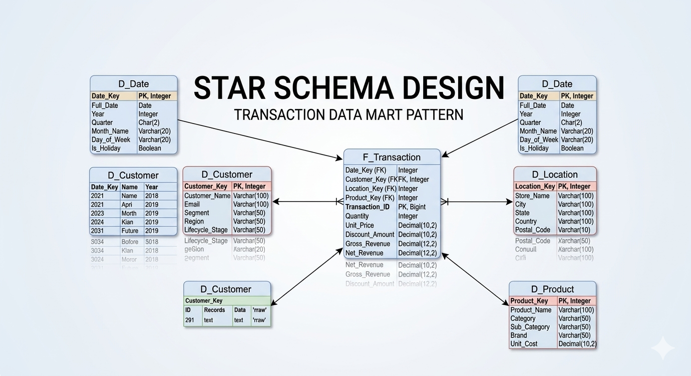
The answer lies in the architectural bedrock of the modern data warehouse: The Star Schema.

Over the last 13 years, I’ve architected data platforms across government, banking, and pension sectors. I have seen every flavor of data modeling, and I can tell you this: the industry has matured, tools have evolved (hello, Spark and distributed compute), but the fundamental rules of physical data modeling remain the ultimate bottleneck for performance.

Here is my playbook for designing dimension and fact tables that actually perform in the real world.

Dimensions: Keep it Flat, Avoid the Snowflake

When designing dimensions, my rule is simple: I strongly prefer a Star Schema over a Snowflake Schema. I actively avoid building dimensions off of dimensions. Every additional join you introduce into a query path degrades performance, especially in distributed cloud architectures.

A properly designed dimension table must contain three core elements:

The Primary Key (PK): A surrogate key (e.g., D_Client_Key) generated by the data warehouse. This is a meaningless integer used exclusively for joining to the fact table.

The Business Key (BK): The natural key from the source system (e.g., Client_ID). This defines the unique record within the dimension and drives your SCD logic.

The Attributes: The descriptive fields associated with that Business Key (e.g., Client_Name, Gender, Birth_Date).

The “Multiple Address” Snowflake Dilemma

While I avoid snowflaking, data modeling requires pragmatism. What happens when a client has multiple addresses (e.g., a Home Address and a Billing Address)?

Some architects will normalize this by creating a D_Address table and snowflaking it off the D_Client table via Foreign Keys (FKs). If the address dimension is very small, this might be acceptable. However, I generally advocate for linking addresses directly to the Fact table.

If we are processing a Billing Fact, the Billing_Address_Key belongs directly on that fact record. Even if that address data is technically duplicated as an attribute within the D_Client table, placing the key on the fact table is superior. It ensures that any measures or mapping attributes tied specifically to that billing event are captured at the correct grain, without forcing the reporting engine to traverse through the client dimension to find where the bill was sent.

Facts: Defining the Grain and Enforcing Purity

The Fact table is the numerical engine of your data model. It should consist entirely of Foreign Keys (pointing to your dimension tables) and Measures (the quantifiable metrics of the business event).

The Golden Rule: No Strings Allowed

Avoid having strings, descriptive text, or categorical attributes within the fact table. Those belong in a dimension. If you find a Transaction_Type_Name varchar column in your fact table, your model is leaking. Move it to a dimension, replace it with a Transaction_Type_Key integer, and watch your storage footprint shrink and your scan speeds soar.

Defining the Grain

The most critical decision in fact table design is defining its grain—what exactly does one single row represent? The grain is driven by the Fact’s Business Key. Is one row a single item on a receipt? Is it the entire receipt? Is it a daily snapshot of an account balance? If you do not explicitly define and document the grain of the fact, you will inevitably end up with double-counting errors in your BI layer.

Scale and Performance: Partitioning the Details

When dealing with massive datasets—such as 200+ million row fact tables—a pristine Star Schema is not enough on its own. You must engineer for the physical realities of data retrieval.

Detail-level facts will inevitably accumulate massive amounts of historical records that are no longer required for day-to-day operational reporting. To alleviate performance bottlenecks, partitioning is mandatory. By physically partitioning the fact table (most commonly by a Date_Key or Month_ID, or occasionally by a specific regional/business grain column), you allow the query engine to perform “partition pruning.” If an analyst queries the last 30 days of data, the database completely ignores the physical files containing the last 5 years of history. When combined with proper indexing strategies, partitioning is the difference between a dashboard loading in 2 seconds versus 2 minutes.

Summary Facts: Designing for the Executive View

Even with perfect partitioning, calculating Year-over-Year (YoY) performance metrics or seasonality trends on the fly from a 200-million-row detail fact table is computationally expensive. Executive KPI dashboards demand sub-second response times, and scanning millions of rows of atomic data will never achieve that.

This is where Summary Fact Tables become critical. As an architect, I routinely design aggregated fact tables at a summarized grain (e.g., Monthly Sales by Region, rather than Individual Transactions). These summary tables act as the high-speed caching layer for your most critical, high-level dashboards, leaving the detail-level fact tables reserved for deep-dive exploratory analytics.

Pragmatism Over Purity: The Architect’s True Job

I want to end with a controversial, yet vital, philosophy: A data model may look “beautiful” on an ERD, but if the performance of the dashboards and reports is poor, the model has failed.

Too often, data modelers try to keep their Star Schemas academically “pure.” They refuse to calculate derived measures in the database, forcing the front-end BI developers (using DAX or Tableau calculations) to do the heavy lifting at runtime.

A clean, performance-driven design must allow for both elegance and brute force. Front-end developers should ask the data modeler to pre-calculate heavy measures within the Star Schema. As a Data Architect, it is your job to actively work with the BI team. You must check in on them to ensure your design is actually meeting their physical needs.

You must avoid creating architectures that rely on multiple, heavy semantic calculation layers between the Gold data model and the final report. Shift the computation left. Do the heavy lifting once during the ETL/ELT pipeline so that a thousand end-users don’t have to wait for it to happen at runtime.

Data modeling is not an academic exercise; it is an engineering discipline meant to serve the business.